Outputs and Visualization

After the execution of the surfatt_tomo, the outputs of the tomography are stored in the directory that is specified in the input parameter file. The outputs include the following files:

Output files

Required outputs

• final_model.h5: The final model file that contains the S-wave velocity model with following attributes:

  • vs: S-wave velocity model in km/s, with the shape of (nx, ny, nz)

  • lon: Longitude of the model in degree with the shape of (nx)

  • lat: Latitude of the model in degree with the shape of (ny)

  • depth: Depth of the model in km with the shape of (nz)

• objective_function.csv: The objective function value of each iteration during the inversion process. The columns are:

  • Iteration number

  • Misfit value

  • Step length

Optional outputs (verbose_level > 0)

• model_iter.h5: The model file of each iteration during the inversion process. The file contains the attributes:

  • vs_{xxx}: S-wave velocity model of iteration {xxx} in km/s, with the shape of (nx, ny, nz)

  • gradient_{xxx}: Preconditioned gradient of iteration {xxx}, with the shape of (nx, ny, nz)

  • direction_{xxx}: Descent direction using CG and LBFGS method of iteration {xxx}, with the shape of (nx, ny, nz)

  • kdensity_{ph}_{xxx}: Kernel density of phase {ph} (available for ph or gr) of iteration {xxx}, with the shape of (nx, ny, nz)

  • lon: Longitude of the model in degree with the shape of (nx)

  • lat: Latitude of the model in degree with the shape of (ny)

  • depth: Depth of the model in km with the shape of (nz)

Optional outputs (verbose_level > 1)

• src_rec_file_{ph}_forward.csv: The forward simulated travel-time data file of phase {ph}

Note

writing this file is time-consuming and memory-consuming, so it is recommended to set verbose_level to 1 for large-scale inversion.

Visualization

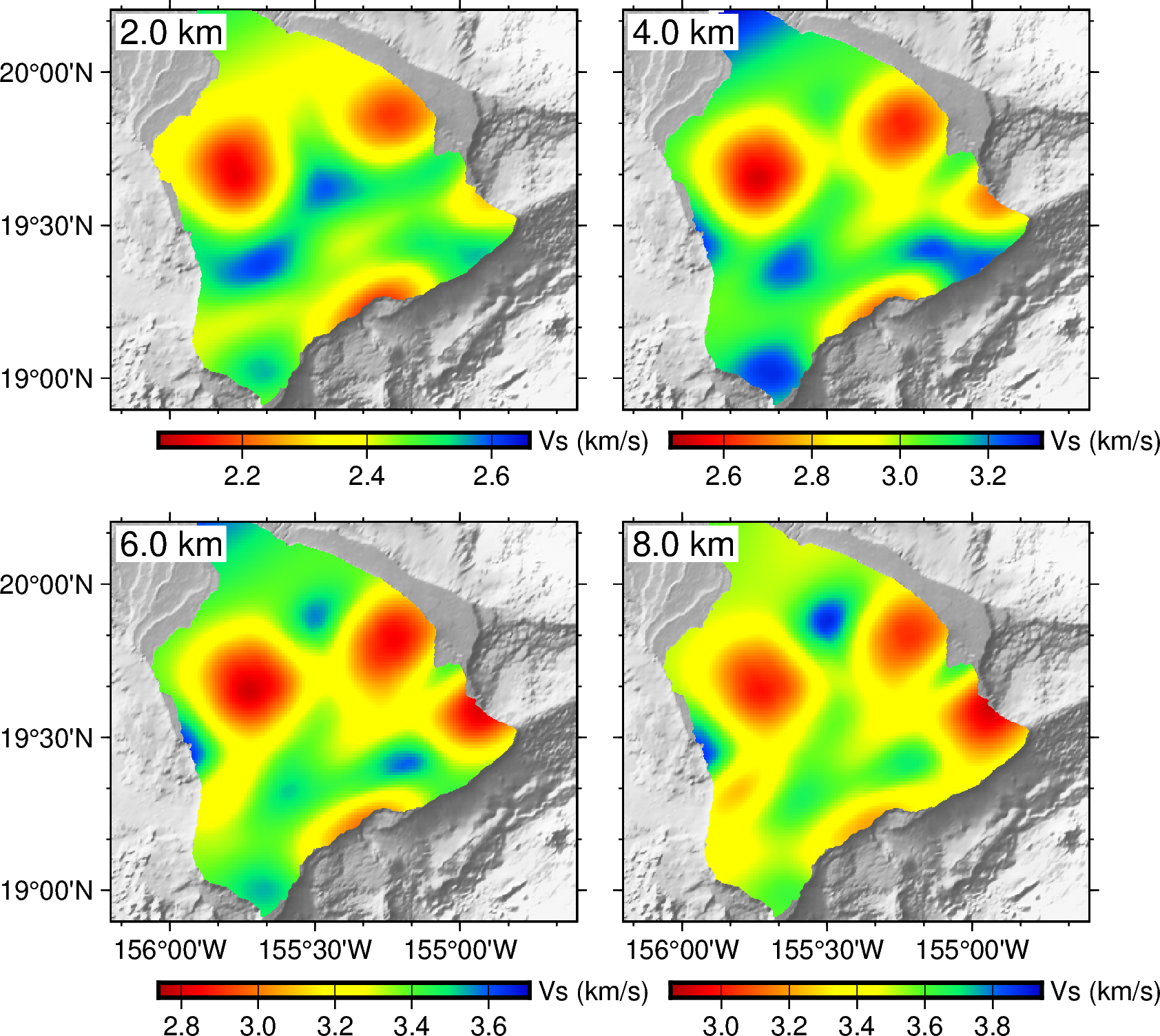
we recommend using the PyGMT package to visualize the outputs of the tomography. Please refer to examples/xxxx/plot_model.ipynb for examples to visualize the final model.

Rotate the model back to the original coordinate system

If the topography, the sources, and the receivers are rotated before the inversion, you can use the surfatt_rotate_model command to rotate the model back to the original coordinate system. The command is called as follows:

Usage: surfatt_rotate_model -i model_file -a angle -c clat/clon -o out_model_file [-h]
 
 Rotate model by a given angle (anti-clockwise) and convert to csv format. If angle and center location are not provided, the model will be converted to csv format directly without rotation
 
 required arguments:
  -i model_file        Path to model file in netcdf format
  -o out_file          Output file name
 
 optional arguments:
  -a angle             Angle in degree to rotate model
  -c clat/clon         Center of rotation in latitude and longitude
  -h                   Print help message

For the Hawaii example, we can rotate the final model back to the original coordinate system using the following command:

angle_back=30
pos_str=19.5/-155.5

surfatt_rotate_model -i OUTPUT_FILES/final_model.h5 -a $angle_back -c $pos_str -o OUTPUT_FILES/final_model.csv

The rotated model is stored in the final_model.csv file with 4 columns: lat, lon, depth, and vs.

The following is an example script to visualize the final model by reading this final_model.csv:

import pygmt
import numpy as np
import pandas as pd

# Load the final model
fm_tab = pd.read_csv("./OUTPUT_FILES/final_model.csv")
z = np.unique(fm_tab["dep"].values)

# Plot the final model
fig = pygmt.Figure()
region=[-156.2, -154.6, 18.9, 20.2]
dep = [2, 4, 6, 8]
pygmt.config(MAP_FRAME_TYPE="plain")
with fig.subplot(nrows=2, ncols=2, figsize=("12c", "12c"), sharex='b', sharey='l', frame=["af", "WSne"]):
    for i, depth in enumerate(dep):
        close_dep = z[np.abs(z-depth).argmin()]
        data = fm_tab[fm_tab["dep"]==close_dep]
        fig.basemap(region=region, projection="M?", panel=i)
        grid = pygmt.grdcut("@earth_relief_15s", region=region)
        pygmt.makecpt(cmap="gray", series=[-6000, 9000, 10], reverse=True)
        fig.grdimage(grid, region=region, projection="M?", cmap=True, shading=True)
        grid = pygmt.surface(x=data['lon'], y=data['lat'], z=data['vs'], region=region, spacing="0.01" )
        vmax = data['vs'].max()+0.05; vmin = data['vs'].min()-0.05
        pygmt.makecpt(cmap="seis", series=[vmin, vmax])
        fig.coast(area_thresh=10, resolution='f', land=True)
        fig.grdimage(grid=grid, cmap=True)
        fig.coast(Q=True)
        fig.text(text=f'{close_dep} km', position='TL', justify='TL', offset='0.1c/-0.1c', fill='white', font='12p')
        fig.colorbar(frame=['a0.2g0.2', 'y+l"Vs (km/s)"'])
fig.show()